#82-How to make an automated attendance sheet in excel with formula(2019) (V2.0)

How to make an automated attendance sheet in excel with formula(2019) (V2.0)

In this tutorial, you can learn How to create a monthly attendance sheet. This is an automated attendance sheet as you read in the title. so with wasting any time let's begin the tutorial......

Creating Helper Sheet

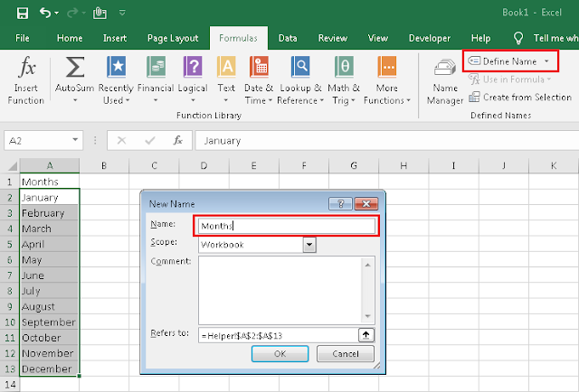
1. Rename the first sheet as Helper then in cell A1 Type Months and on Cell A2 Type January. Then drag the fill handle of cell A2 up to A13

              

Then select from January to December and Click on Define Name in Formula Tab. Type Months in the name box and click OK.

2. In Cell C2 type Holidays, then in the C column type the name of the holidays, and in column D type the dates of the holidays.

Then create Named Range for the holiday list. Select the dates, then click the Define Name in the Formula tab. Type Holidays in the Name box and click OK.

Creating Attendance Sheet

Create a new sheet and rename it as Attendance. 

1) Creating Attendance Header

a) In A1 type Attendance for the Month of then select cell from A1 to L1 and click on  Merge & Center

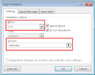
b)  Select cell M1 to Q1 and Merge it, then here create a dropdown list of Month. Goto Data tab then select Data Validation. In the Allow box select List, then click on Source box and press F3 and select Month  and click OK again OK.

c) Select cell R1 to T1 and Merge it. 

then here create a dropdown list of Month. Goto Data tab then select Data Validation. In the Allow box select List, then click on Source box and type 2019,2020,2021,2022 and click OK.

 

2) Creating Dates

a) In C2 type Start Date and H2 type End Date. Merger the cells from D2 to F2 and cells from I2 to K2.

b) In cell D2 type the formula =DATEVALUE("1"& M1&R1) and on I2 type the formula =EOMONTH(D2,0).

 c)  Format the cell D2 and I2 to short date.

3) Creating Employee ID and Names

a) Merge the cells A5 and A6 and type Emp ID.

b) Merge the cells B5 and B6 and type Employee Name.

c)  Then type the Employee ID and Employee Name as shown in the image below.

4) Creating Date Row & Day Row

a) In cell C6, type the formula =D2 for the first date in the date row.

b) In cell  D6, type the formula =IF(C5<$I$2,C6+1,""), then drag the fill handle of D5 till AG column.

c) Select the column from C to AG and change the column width to 3.5. 

d) In  C5 type the formula =TEXT(C5,"ddd"), then drag the fill handle of C4 till AG column.

 5) Create Report Heads

a) Merge the cells AH5 & AH6, AI5 & AI6, AJ5 & AJ6, AK5 & AK6, AL5 & AL6, AM5 & AM6
b) Type Full Day Present in AH5, Full Day Absent in AI5, Half Day in AJ5, Work Days in AK5, Pr. Percent in AL5, Ab. Percent in AM5.

6) Creating Holiday Helper Row

a) In cell C4 type the formula =IFERROR(IF(C6="",1,MATCH(C6,Holidays,0)),0) 
b)  Drag the fill hand of cell C4  till the last date.

 7) Highlight Weekend with Conditional Formatting

a) Select cell C5 to AG6, and Goto Home → Conditional Formatting → New Rule
b) Select Use a formula to determine which cells to format
c) in Edit the Rile Description box type the formula =OR(C$5="sun") 
Hint: If you want both Sat & Sun as Weekend then =OR(C$5="sat",C$5="sun")
d) Then click Format and choose the formatting according to your choice, then OK and again OK.
e) Select the Attendance area and repeat the same step. 

8) Highlight Holidays with Conditional Formatting

a) Select cell C5 to AG6, and Goto Home → Conditional Formatting → New Rule
b) Select Use a formula to determine which cells to format
c) in Edit the Rile Description box type the formula =COUNTIF(Holidays,C$6) 
d) Then click Format and choose the formatting according to your choice, then OK and again OK.
e) Select the Attendance area and repeat the same step. 

9) Do the rest of the formatting according to your choice or watch the video given at the top.

10) Data Validation to Restrict cell for attendance entry

a) Select the attendance area, then Go to Data → Data Validation

b) In Allow box select Custom

c) In Formula box type =C$6<>""  and Click OK.

11) Formula for Report Part

a) Formula for Present: =COUNTIFS(C7:AG7,"P",$C$5:$AG$5,"<>Sun",$C$4:$AG$4,0)

b) Formula for Absent: =COUNTIFS(C7:AG7,"A",$C$5:$AG$5,"<>Sun",$C$4:$AG$4,0)

c) Formula for Hald Day: =COUNTIFS(C7:AG7,"H",$C$5:$AG$5,"<>Sun",$C$4:$AG$4,0)

d) Formula for Workdays: =COUNTIFS($C$5:$AG$5,"<>Sun",$C$4:$AG$4,0)

e) Formula for Present Percent: =(AH7+AJ7*0.5)/AK7   & Format as Percent

f) Formula for Absent Percent: =AI7/AK7  & Format as Percent

g) Drag all the formulas down.

12) Create buttons for COPY SHEET & CLEAR SHEET

a) Goto Insert → Illustrations → Shapes then select Rectangle

b) Draw the rectangle then make another copy of it and edit the text in each shape as COPY SHEET & CLEAR SHEET respectively.

c) Format then as your choice or see the video.

13) Creating VBA Macro for Copy Sheet

a) Press ALT+F11

b) Click Insert →  Module

c) Type the following codes

Sub Copyrenameworksheet()

    Dim ws As Worksheet

    Set wh = Worksheets(ActiveSheet.Name)

    On Error Resume Next

    ActiveSheet.Copy After:=Worksheets(Sheets.Count)

    If wh.Range("A1").Value <> "" Then

    ActiveSheet.Name = wh.Range("M1").Value

   

    End If

    wh.Activate

End Sub

14) Create VBA Macro for Clear Sheet

a) Type the following codes

Sub Clearcells()

Range("C7", "C16").ClearContents

Range("D7", "D16").ClearContents

Range("E7", "E16").ClearContents

Range("F7", "F16").ClearContents

Range("G7", "G16").ClearContents

Range("H7", "H16").ClearContents

Range("I7", "I16").ClearContents

Range("J7", "J16").ClearContents

Range("K7", "K16").ClearContents

Range("L7", "L16").ClearContents

Range("M7", "M16").ClearContents

Range("N7", "N16").ClearContents

Range("O7", "O16").ClearContents

Range("P7", "P16").ClearContents

Range("Q7", "Q16").ClearContents

Range("R7", "R16").ClearContents

Range("S7", "S16").ClearContents

Range("T7", "T16").ClearContents

Range("U7", "U16").ClearContents

Range("V7", "V16").ClearContents

Range("W7", "W16").ClearContents

Range("X7", "X16").ClearContents

Range("Y7", "Y16").ClearContents

Range("Z7", "Z16").ClearContents

Range("AA7", "AA16").ClearContents

Range("AB7", "AB16").ClearContents

Range("AC7", "AC16").ClearContents

Range("AD7", "AD16").ClearContents

Range("AE7", "AE16").ClearContents

Range("AF7", "AF16").ClearContents

Range("AG7", "AG16").ClearContents

End Sub

or

Sub Clearcells()

Range("C7:AG16").ClearContents

End Sub

15) Assigning Macros to the buttons

a) Right-click on the COPY SHEET button and click Assign Macro then the macro copyrenameworksheet

b) Right-click on the COPY SHEET button and click Assign Macro then the macro Clearcells

c) Click OK

If you face any problem you can watch the video at the top and you can also comment me if you did not find the solution to your problem.

That's All

********************************* ~:Support Our Work Financially:~ *********************************

Project File Type: Premium

Project File Cost: Rs.100/-

************************************************************************************************